Welcome to the regression section of the Python Machine Learning series. By now, you should have Scikit-Learn installed. If not, make sure to install it along with Pandas and Matplotlib for data manipulation and visualization.
Use the following commands to install the necessary packages:
pip install numpy
pip install scipy
pip install scikit-learn
pip install matplotlib
pip install pandas
Additionally, we will be using Quandl for financial data. Install it with:
pip install quandl
Regression is a fundamental technique in machine learning that deals with predicting continuous values. The goal is to find the best-fit equation that models the relationship between input variables and a target variable. With simple linear regression, this can be done by fitting a straight line to the data points.
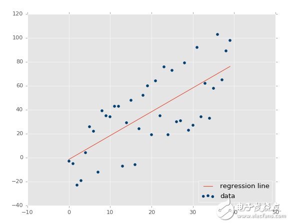
This line can then be used to predict future values, such as stock prices, where time (date) is on the x-axis.
One of the most common applications of regression is in forecasting stock prices. Since stock prices are time-dependent and involve continuous data, regression helps us predict the next price based on historical patterns.
Regression is a type of supervised learning, meaning that the model is trained using labeled data—where both input features and the corresponding correct output are provided. After training, the model is tested on unseen data to evaluate its performance. If the accuracy is satisfactory, it can be deployed in real-world scenarios.
To start with an example, we'll use stock market data from Quandl. We'll fetch Google's stock data using the symbol GOOGL:
import pandas as pd
import quandl
df = quandl.get("WIKI/GOOGL")
print(df.head())
Note: At the time of writing, Quandl uses lowercase 'q' for its module, so ensure you import it correctly.
The dataset includes several columns such as Open, High, Low, Close, Volume, and adjusted prices. Here’s a sample of the data:
Open | High | Low | Close | Volume | Ex-Dividend | Split Ratio | Adj. Open | Adj. High | Adj. Low | Adj. Close | Adj. Volume
Date
2004-08-19 | 100.00 | 104.06 | 95.96 | 100.34 | 44659000 | 0 | 50.000 | 52.03 | 47.980 | 50.170 | 44659000
2004-08-20 | 101.01 | 109.08 | 100.50 | 108.31 | 22834300 | 0 | 50.505 | 54.54 | 50.250 | 54.155 | 22834300
We see that some columns like 'Adj. Open' and 'Open' are duplicates, but the adjusted prices are more useful for analysis because they account for stock splits and other corporate actions.
To simplify our dataset, we’ll keep only the adjusted columns:
df = df[['Adj. Open', 'Adj. High', 'Adj. Low', 'Adj. Close', 'Adj. Volume']]
Now we have a cleaner dataset. However, raw data alone isn't enough. Machine learning models rely on meaningful features. For example, instead of just using the open, high, low, and close prices, we can calculate daily changes, volatility, or percentage differences to extract more valuable insights.
Understanding the data is key. Not all data is useful, and sometimes less is more. Feature engineering—transforming raw data into meaningful features—is essential for building accurate models. In the next steps, we’ll explore how to prepare these features for regression analysis.
ZHOUSHAN JIAERLING METER CO.,LTD , https://www.zsjrlmeter.com