Modeling and Simulation of Microwave Equalizer Based on Neural Network
High power traveling wave tubes and other microwave tubes are the core devices of radar and other electronic equipment, and their technical level determines the tactical performance of electronic equipment. However, due to the large gain fluctuation of the high-power microwave tube, under the condition of equal excitation input, all points in the frequency band cannot be saturated, which will cause harmonics and intermodulation components in the input signal, resulting in the defective rate of the microwave vacuum tube. The rise, more importantly, directly affects the performance of modern electronic equipment, especially difficult to meet the high environmental reliability requirements of modern warfare. Therefore, it is necessary to use high-power microwave tube equalization technology, that is, to add a microwave network to make its transmission characteristics compensate for the transmission characteristics of the microwave tube, so that the output power fluctuation of the traveling wave tube is minimized.
The equalizer with multi-cavity structure is a device with a complex microwave structure. Due to the complexity of its structure, its strict mathematical representation is very complicated. Whether it is analytical or numerical, it is difficult to solve directly. The calculation results of the non-ideal factors simplified are too large, and the practical value is not high. Under the condition that the accurate electromagnetic characteristics cannot be obtained, the debugging work cannot be effectively guided, and the optimal design can not be discussed. This problem is also ubiquitous for the complex microwave structures commonly used in microwave engineering at present, and is also a problem that needs to be solved urgently. Therefore, in order to increase the design speed and save design costs, the equalizer is modeled for computer-aided Design is becoming more and more important.
The transmission characteristics of the microwave equalizer are mainly determined by its structural size and frequency. They form a nonlinear mapping relationship, and the neural network can quickly and accurately simulate any linear and nonlinear functional relationship, and has a good association ability. . Therefore, artificial neural networks can be used to model the equalizer. Although the neural network training process takes a certain amount of time, once the neural network model is trained, the results can be obtained in a short time without sacrificing accuracy. Therefore, the use of neural network models to assist in the design of microwave equalizers will Will greatly improve the design speed and save debugging time.
1 Basic single-cavity sub-structure of the equalizer Figure 1 is a single sub-structure diagram of the absorption coaxial microwave amplitude equalizer. The cascade of multiple sub-structures is based on this. One end of the coaxial resonant cavity is connected to the main transmission line, and the other end is an adjustable short-circuit piston, which can adjust the length of the resonant cavity. The resonant cavity is an adjustable coupling probe inserted into the main transmission line, and the energy in the main transmission line is passed through the probe Coupling into the resonant cavity, changing the resonant cavity length and probe insertion depth can adjust the resonant frequency and quality factor Q value of the resonant cavity. In addition, an attenuation rod made of absorbing material can also be inserted at an appropriate position on the side wall of the resonant cavity. 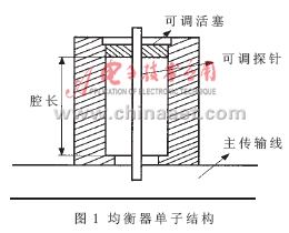
However, due to the limitation of the bandwidth of the single sub-structure and the amplitude of absorption and attenuation, in order to achieve high-precision equalization of high-power microwave tubes in a wider frequency band, a multi-level sub-structure cascade must be adopted. Therefore, in engineering practice, a network substructure interconnection analysis method based on massive database is proposed for the complex characteristics of the equalizer. During the establishment of the database, the network analyzer was used to measure the S-parameters of the single-chamber sub-structure of the equalizer, and the corresponding S-parameter measurement database was established. The physical parameters of the equalizer corresponding to each measurement point in this database are: the cavity length Lc of the resonant cavity, the depth of the coupling line inserted into the transmission line Ls, and the dielectric perturbation inserted into the depth of the resonant cavity La. It can be known from engineering practice that the influence of three physical parameters on the frequency of the resonance frequency point can be followed regularly. Generally, the resonant frequency decreases with increasing Lc; the resonant frequency decreases with increasing Ls and the attenuation increases at the same time; the resonant frequency decreases with increasing La and the attenuation decreases at the same time.
2 Design of neural network model
2.1 RBF neural network RBF (Radius Base FuncTIon) is a new type of neural network that has emerged in the last decade. It has a simple network structure and fast network training speed (compared to the BP algorithm, the training algorithm of the RBF network can be an order of magnitude faster) , High simulation accuracy and other advantages. RBF network also has good locality, can provide smooth, excellent performance of discrete data interpolation characteristics, the system composed of the network is bounded and stable.
The structure of the RBF neural network is shown in Figure 2. It is a two-layer network. The first layer consists of RBF neurons as hidden neurons (the transfer function is a Gaussian function). In the figure, a1i represents the i-th element of vector a1 ; B1i represents the i-th element of the vector b1 (that is, the variance of the i-th RBF neuron); iW1 represents the i-th row of the matrix W1, that is, the center of the i-th neuron. The second layer consists of linear neurons (the transfer function is a linear function) as output neurons. Where S1 and S2 represent the number of neurons in the first and second layers, respectively. 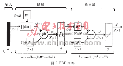
If you consider the case of S2 = 1, then consider the entire neural network as a 
Where ci (i = 1,2, ..., S) is each row of matrix C, which represents the center vector of the radial basis function of the corresponding neuron, b1 = λ = (λ1, λ2, ... λS), where λi represents The variance of the radial basis function, W2 = W = (w1, w2, ..., wS), then the network output is: 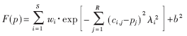
2.2 Network training It is meaningless to build such a model. The neural network must learn before actual work. Through learning, the neural network can obtain certain "intelligence".
Learning is one of the most important and remarkable features of neural networks. In the development of neural networks, the study of learning algorithms has a very important position. At present, the neural network models proposed by people all correspond to learning algorithms. Therefore, sometimes people do not demand strict definition or distinction between models and algorithms. Some models can have multiple algorithms, and some algorithms may be used in multiple models.
In this paper, according to the transmission characteristics of the equalizer, during the training and learning process, the continuous adjustment of the connection weight and the correction of the learning adopt the LM algorithm in the BP network learning algorithm. The LM algorithm is the fastest algorithm proposed for training a medium-scale feed-forward neural network. It is also very effective for MATLAB implementation. Among the many learning algorithms of the BP network, it is usually close to the network for functions containing hundreds of weights. The LM algorithm has the fastest convergence speed. If the required accuracy is relatively high, the advantages of this algorithm are particularly prominent. In many cases, the training function trainlm using the LM algorithm can obtain a smaller mean square error than other algorithms.
LM algorithm is actually a combination of gradient descent method and Newton method. Gradient descent method descents faster in the first few steps. When the gradient is close to the optimal value, the objective function declines slowly because the gradient tends to zero; Newton's method can produce an ideal search direction near the optimal value. The main algorithm is: 
Where J is the Jacobian matrix containing the first derivative of the network error versus weight and threshold.
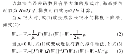
Newton's method can approach a minimum error more quickly and accurately. After each step is successful, μ will decrease, and only increase when the output is found to be bad in the next step. In this way, each step of the algorithm will make the objective function develop in a good direction.
At the beginning of the algorithm, μ takes a small value μ = 0.001. If E cannot be reduced by a certain step, multiply μ by 10 and repeat this step, and finally decrease E. If a smaller step produces a smaller E, then multiply μ by 0.1 to continue. The execution steps of the algorithm are shown in Figure 3. 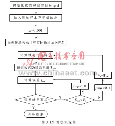
The main difference between the RBF network and the BP network is the use of different function functions. The hidden nodes in the BP network use the Sigmoid function, whose function value is a non-zero value in an infinite range in the input space. The function of the RBF network is a Gaussian function, so it has the characteristic that the Gaussian function value is greater than zero for any input, thus losing the advantage of adjusting the weight. However, after adding the LM algorithm for network training, the RBF network also has the advantage of fast learning convergence of the local approximation network, which can overcome the shortcomings of the Gaussian function that is not compact. Since the RBF network uses a Gaussian function, the representation form is simple, and even for multivariable input, it does not add too much complexity.
2.3 Simulation design results
In the modeling process, if you want to build an accurate neural network model, you usually need to provide a large number of training samples. In the course of the project, the network substructure interconnection analysis method based on the massive database is proposed for the complex characteristics of the microwave equalizer. The proposal of this method provides a large number of accurate training samples for building the equalizer neural network model.
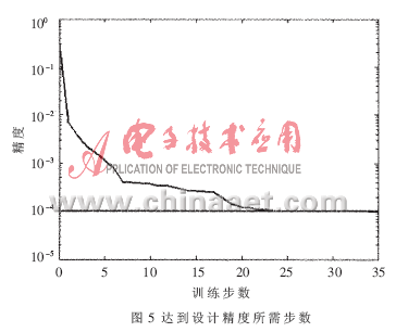
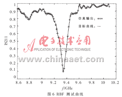
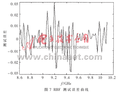
In this paper, the RBF network with LM algorithm for network training is used to model the equalizer, and the structural size of the equalizer (the cavity length of the resonant cavity, the depth of the probe inserted into the main transmission line, the depth of absorption material insertion) and the frequency are used as the neural network ’s Input samples, and S-parameters as output samples for RBF network training. A total of 100 sets of samples were selected as training data, and another 100 sets of samples were selected as test data for the performance of the neural network model. The frequency is 8.6GHz≤freq≤10.092 5GHz. Simulate the relationship between S parameters and input samples: Y = F (X), where: X is the input variable of the neural network; Y is the output variable, Y = (| S11 |, | S21 |). The simulation and training results of | S21 | in the simulation output variables using MATLAB software are shown in Figure 4 to Figure 7. Among them, Figure 4 is the simulation curve of the RBF network, which shows that the error is very small. Figure 5 shows that the number of training steps required to achieve the expected design accuracy of 0.0001 is 35 steps, and this network quickly reaches the design accuracy. In order to verify the performance of the RBF network after training, another 100 samples were selected for testing. The test curve is shown in Figure 6. The test performance of the RBF network can be shown in Figure 7. The absolute value of the test absolute error is less than 0.03, 98% The relative error of the test is less than 5%, and the relative error is greater at the inflection point where the attenuation of | S21 | is greatest. This is because the selection of the test point at the inflection point fails to meet the principle of experimental design (DOE). The simulation output again shows that the performance of RBF neural network modeling is quite stable. Moreover, the results of simulation design using this neural network are very repeatable, and the effect achieved by the design is satisfactory. 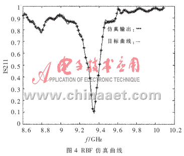
This article uses the RBF neural network to model the microwave equalizer. The results of the simulation design are compared with the test results of the network analyzer, and the error is small. This shows that the neural network model design method proposed in this paper makes the design process of microwave equalizer become faster and more accurate, and has the advantages of accuracy, time saving and auxiliary design. It has good application value for the analysis and design of microwave devices.
| About Film Covered Flat Aluminium Wire |
Fiber glass film covered enameled aluminum flat wire
The product is the premium copper or aluminum to be enameled, then to be wrapped with polyester film or polyimide film so as to enhance the breakdown voltage of enameled wire. It has the advantages of thin insulation thickness, high voltage resistance. The product is the ideal material for electrical instruments of small size, large power, high reliability.

Copper or Aluminum rectangular Wire
Narrow side size a : 1.00 mm-5.60 mm
Broad side size b : 2.00 mm-16.00 mm
Film Covered Flat Aluminium Wire
Film Covered Copper Wire,Film Covered Flat Aluminium Wire,Covered Flat Magnet Wire,Fiberglass Covered Wire
HENAN HUAYANG ELECTRICAL TECHNOLOGY GROUP CO.,LTD , https://www.huaonwire.com